Difference Between Array and Linked List In Data Structure | Unit 1(2) | Aktu DSA Notes | AKTU FREE NOTES

 

Arrays

Definition:

An array is a fundamental data structure that stores elements of the same data type in a contiguous block of memory. Think of it as a dynamic collection of items, each uniquely identified by an index or a key. The power of arrays lies in their ability to organize and efficiently manage data, providing quick access to individual elements based on their position.

1-D Array (GeeksForGeeks)

Single and Multidimensional Arrays:

Single-Dimensional Array:

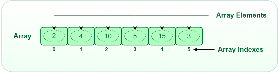
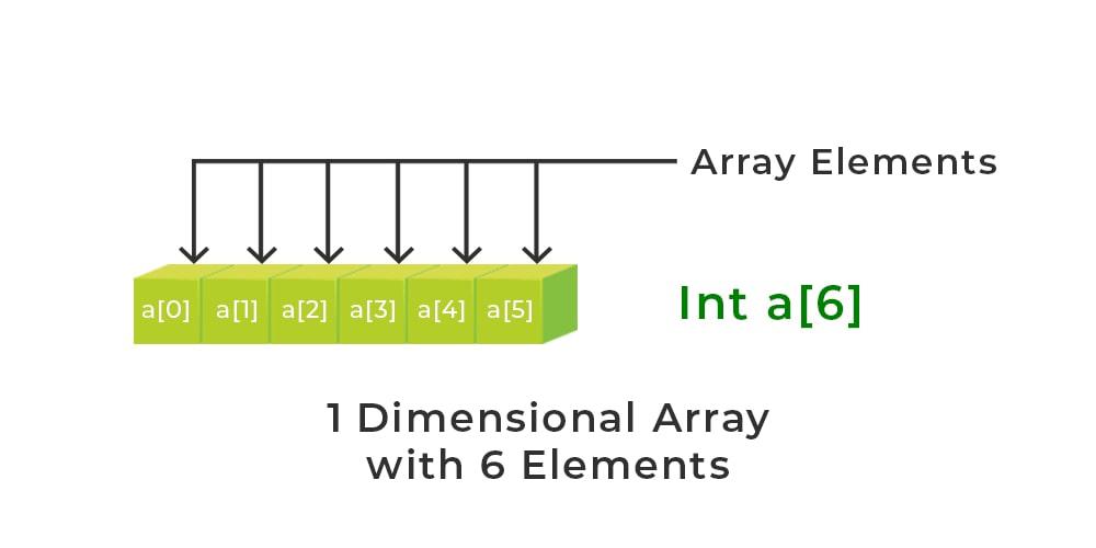
A single-dimensional array is the simplest form of an array, representing a linear list of elements. This structure is akin to a series of connected storage locations, each holding a single data item. The arrangement is sequential, with each element accessed using a single index.

• Simple List Structure:

  • A single-dimensional array can be visualized as a straight line of storage locations.
  • Each element is uniquely identified by its position in the sequence, starting from the first element (index 0) to the last element.

• Example:

  • Let's consider an example array int numbers[5] = {1, 2, 3, 4, 5};.
  • Here, the array numbers contains five integers, and each integer can be accessed by its respective index. For instance, numbers[2] would refer to the element with the value 3.

Multidimensional Arrays:

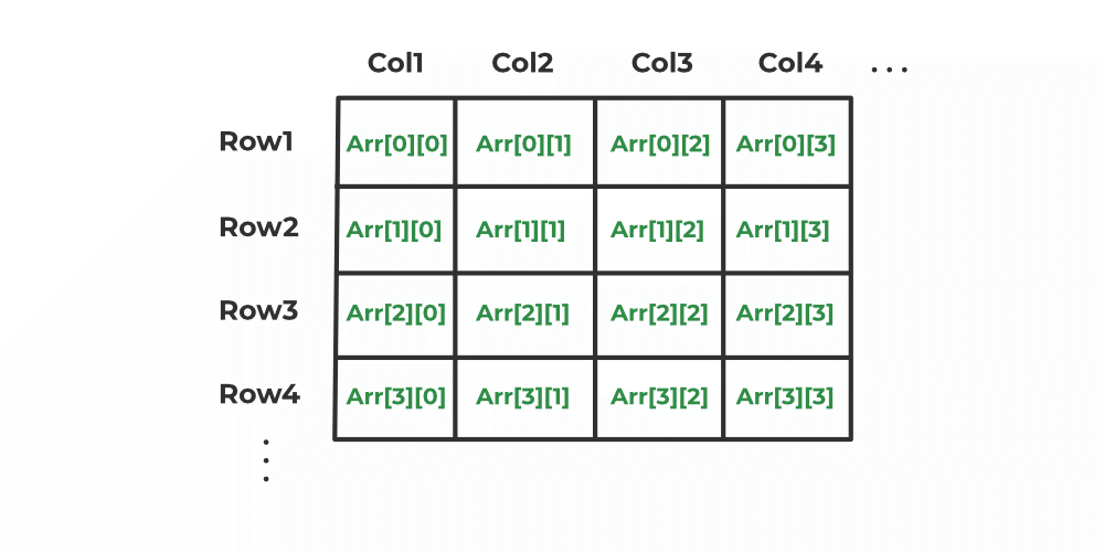
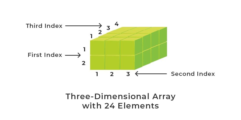
Multidimensional arrays take the concept further by introducing more than one dimension. These arrays create tables or matrices of elements, and each element is identified by multiple indices.

• Arrays with More Than One Dimension:

  • While a single-dimensional array is like a line, a 2D array resembles a grid, and a 3D array can be thought of as a cube, and so on.
  • Each dimension adds a layer of complexity to the data structure.

• Example:

• Consider a 2D array int matrix[3][3] = {{1, 2, 3}, {4, 5, 6}, {7, 8, 9}};.
• In this case, matrix represents a 3x3 grid of integers. Each element is accessed using two indices, representing the row and column, such as matrix[1][2], which refers to the element with the value 6.

• 

  2D Array (Geeksforgeeks)

  
  
  

• Extending to Higher Dimensions:

  • Multidimensional arrays can extend to 3D, 4D, and beyond. Each added dimension introduces a new axis and set of indices.

Practical Insights:

Choosing Between Single and Multidimensional Arrays:

• Single-Dimensional Arrays:

  • Ideal for representing linear sequences of data.
  • Efficient for scenarios where data can be logically arranged in a straight line.

• Multidimensional Arrays:

• Suited for tabular or grid-like data representations.
• Useful when dealing with matrices or structures with multiple dimensions.

Representation of Arrays:

When it comes to storing elements in memory, the order in which they are arranged matters. Two common ways of arranging elements in a multidimensional array are Row Major Order and Column Major Order.

Row Major Order:

In row major order, the elements of a multidimensional array are stored row by row in memory. This means that the entire first row is stored first, followed by the second row, and so on. In the context of a 2D array, the sequence of storage proceeds from left to right across each row before moving on to the next row.

Column Major Order:

In column major order, the elements are stored column by column. For a 2D array, this means storing the elements of the first column, followed by the second column, and so forth. The sequence of storage proceeds from top to bottom down each column before moving on to the next column.

Visualization:

• Consider a 2D array int matrix[3][3] = {{1, 2, 3}, {4, 5, 6}, {7, 8, 9}};.

• 

  Credit: The craft of coding

  
  
  
• In row major order, the memory layout would be: 1, 2, 3, 4, 5, 6, 7, 8, 9.
• In column major order, the memory layout would be: 1, 4, 7, 2, 5, 8, 3, 6, 9.

Calculation of Index:

Let's use the example array int matrix[3][3] = {{1, 2, 3}, {4, 5, 6}, {7, 8, 9}}; to demonstrate the calculation of indices in both Row Major Order and Column Major Order.

Row Major Order:

In Row Major Order, elements are stored row by row. The index calculation for a given element at position (i, j) is:

$\text{index}=(�\times \text{num\_columns})+�$

Let's calculate the indices for a few elements:

1. Element at (0, 1):

   • $\text{index}=(0\times 3)+1=1$
   • So, the element with value 2 is at index 1 in Row Major Order.

2. Element at (2, 0):

   • $\text{index}=(2\times 3)+0=6$
   • So, the element with value 7 is at index 6 in Row Major Order.

Column Major Order:

In Column Major Order, elements are stored column by column. The index calculation for a given element at position (i, j) is:

$\text{index}=(�\times \text{num\_rows})+�$

Now, let's calculate the indices for the same elements:

1. Element at (0, 1):

   • $\text{index}=(1\times 3)+0=3$
   • So, the element with value 2 is at index 3 in Column Major Order.

2. Element at (2, 0):

• $\text{index}=(0\times 3)+2=2$
• So, the element with value 7 is at index 2 in Column Major Order.
• 
  

• 

  Credit: The craft of coding
  
  

  
  

3. Calculation of address of element of 1-D, 2-D, and 3-D using row-major and column-major order

1-D Array:

• Formula: $\text{Address of }�[�]=�+�\times (�-��)$

• $�[�]$: The element in the array at position $�$.
• $�$: Base address, where the array starts.
• $�$: Storage size of one element (in bytes).
• $�$: The position of the element you want to find.
• $��$: Lower bound or starting point of the array (default is zero).
• 
  
  
  
  

Assume we have an array int arr[6] = {10, 20, 30, 40, 50 , 60};.

• Formula: $\text{Address of }���[�]=�+�\times (�-��)$

  • $�$: Base address (let's assume 1000 for this example).
  • $�$: Storage size of one element (let's assume 4 bytes for int).
  • $��$: Lower bound (assuming it starts from zero).

Example: To find the address of arr[2]:

$\text{Address}=1000+4\times (2-0)=1008$

So, the address of arr[2] is 1008.

2-D Array:

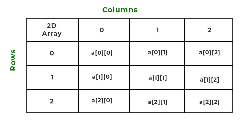2D Array

Row Major Order:

• Formula: $\text{Address of }�[�][�]=�+�\times ((�-��)\times �+(�-��))$

  • $�[�][�]$: The element in the 2D array at row $�$ and column $�$.
  • $�$: Base address, where the array starts.
  • $�$: Storage size of one element (in bytes).
  • $�,�$: Positions of the element you want to find.
  • $��,��$: Lower bounds or starting points of rows and columns (default is zero).
  • $�$: Number of columns in the 2D array.

Column Major Order:

• Formula: $\text{Address of }�[�][�]=�+�\times ((�-��)\times �+(�-��))$

• $�[�][�]$: The element in the 2D array at row $�$ and column $�$.
• $�$: Base address, where the array starts.
• $�$: Storage size of one element (in bytes).
• $�,�$: Positions of the element you want to find.
• $��,��$: Lower bounds or starting points of rows and columns (default is zero).
• $�$: Number of rows in the 2D array.

Assume we have a 2D array int matrix[3][4] = {{1, 2, 3, 4}, {5, 6, 7, 8}, {9, 10, 11, 12}}.

Row Major Order:

• Formula: $\text{Address of }������[�][�]=�+�\times ((�-��)\times �+(�-��))$

  • $�$: Base address (let's assume 2000 for this example).
  • $�$: Storage size of one element (let's assume 4 bytes for int).
  • $��,��$: Lower bounds (assuming they start from zero).
  • $�$: Number of columns (4 in this case).

Example: To find the address of matrix[1][2]:

$\text{Address}=2000+4\times ((1-0)\times 4+(2-0))=2012$

So, the address of matrix[1][2] is 2012.

Column Major Order:

• Formula: $\text{Address of }������[�][�]=�+�\times ((�-��)\times �+(�-��))$

  • $�$: Base address (let's assume 2500 for this example).
  • $�$: Storage size of one element (let's assume 4 bytes for int).
  • $��,��$: Lower bounds (assuming they start from zero).
  • $�$: Number of rows (3 in this case).

Example: To find the address of matrix[1][2]:

$\text{Address}=2500+4\times ((2-0)\times 3+(1-0))=2516$

So, the address of matrix[1][2] is 2516.

3-D Array:

Assume we have a 3D array int cube[2][3][4] = {{{1,2,3,4}, {5,6,7,8}, {9,10,11,12}}, {{13,14,15,16}, {17,18,19,20}, {21,22,23,24}}.

Row Major Order:

• Formula: $\text{Address of }����[�][�][�]=�+�\times (�\times �\times (�-�)+�\times (�-�)+(�-�))$

  • $�$: Base address (let's assume 3000 for this example).
  • $�$: Storage size of one element (let's assume 4 bytes for int).
  • $�,�,�$: Lower bounds (assuming they start from zero).
  • $�,�,�$: Number of rows, columns, and width (2, 3, 4 in this case).

Example: To find the address of cube[1][2][3]:

$\text{Address}=3000+4\times (2\times 3\times (1-0)+3\times (2-0)+(3-0))=3056$

So, the address of cube[1][2][3] is 3056.

Column Major Order:

• Formula: $\text{Address of }����[�][�][�]=�+�\times (�\times �\times (�-�)+�\times (�-�)+(�-�))$

  • $�$: Base address (let's assume 3500 for this example).
  • $�$: Storage size of one element (let's assume 4 bytes for int).
  • $�,�,�$: Lower bounds (assuming they start from zero).
  • $�,�,�$: Number of rows, columns, and width (2, 3, 4 in this case).

Example: To find the address of cube[1][2][3]:

$\text{Address}=3500+4\times (2\times 3\times (1-0)+2\times (3-0)+(2-0))=3564$

So, the address of cube[1][2][3] is 3564.

Dynamic Arrays:

A dynamic array, also known as a resizable array or an ArrayList in some programming languages, is a data structure that provides a flexible and dynamic approach to working with arrays. Unlike static arrays, which have a fixed size at the time of declaration, dynamic arrays can grow or shrink in size during program execution.

Characteristics of Dynamic Arrays:

1. Resizable Size:

   • One of the key features of dynamic arrays is that they can dynamically resize themselves during runtime.
   • This allows for efficient memory utilization, as the array can be adjusted to accommodate the actual number of elements.

2. Efficient Random Access:

   • Dynamic arrays support constant-time random access to elements, just like static arrays.
   • Elements are stored in contiguous memory locations, allowing direct access based on indices.

3. Contiguous Memory Allocation:

   • Similar to static arrays, dynamic arrays allocate memory in a contiguous block.
   • This enables efficient traversal and access, making them suitable for tasks requiring quick access to elements.

4. Automatic Memory Management:

   • Dynamic arrays handle memory management automatically, abstracting the complexity of memory allocation and deallocation from the programmer.
   • When the array needs to grow beyond its current capacity, a new, larger memory block is allocated, and existing elements are copied over.

How Dynamic Arrays Work:

1. Initialization:

   • A dynamic array is initialized with a small initial capacity (e.g., 10 elements).
   • The array keeps track of its current size and capacity.

2. Adding Elements:

   • When an element is added to the array and the current size exceeds the capacity, a new, larger memory block is allocated.
   • Existing elements are copied to the new block, and the new element is added.

3. Removing Elements:

• When an element is removed, and the size drops below a certain threshold, the array may be resized to a smaller capacity to save memory.
• The process involves allocating a new block with reduced capacity and copying elements.
4. 
   
5. 

   
   
   
   
   
   

Advantages of Dynamic Arrays:

1. Flexibility:

   • Dynamic arrays provide flexibility in handling varying amounts of data.

2. Efficient Operations:

   • Efficient random access and memory utilization make dynamic arrays suitable for a wide range of applications.

3. Automatic Memory Management:

   • Automatic resizing and memory management reduce the burden on the programmer.

Disadvantages of Dynamic Arrays:

1. Overhead:

   • Dynamic arrays may incur additional overhead due to resizing and copying elements.

2. Fragmentation:

   • Over time, dynamic arrays may lead to memory fragmentation as old memory blocks become unused.

Use Cases:

1. Lists and Collections:

   • Dynamic arrays are commonly used to implement lists, vectors, and other resizable collections.

2. Database Implementations:

   • In scenarios where the number of records can vary, dynamic arrays provide an efficient way to manage data.

3. String Manipulation:

• Dynamic arrays are useful for operations involving string concatenation and manipulation.

Operations On Array:

1. Insertion Operation:

Algorithm:

1. Input: Array arr, its current size n, index pos where the element is to be inserted, and the value val to be inserted.
2. Validation: Check if pos is a valid index (0 <= pos <= n).
3. Shift Elements:
   • Starting from the last element, shift elements to the right to make space for the new element.
   • Repeat until reaching the position pos.
4. Insert Element: Place the value val at the position pos.
5. Update Size: Increment the size n by 1.

Definition:

Insertion in an array involves adding an element at a specified position, shifting existing elements to make room for the new element.

2. Deletion Operation:

Algorithm:

1. Input: Array arr, its current size n, and index pos of the element to be deleted.
2. Validation: Check if pos is a valid index (0 <= pos < n).
3. Shift Elements:
   • Starting from the position pos, shift elements to the left to fill the gap left by the deleted element.
   • Repeat until reaching the last element.
4. Update Size: Decrement the size n by 1.

Definition:

Deletion in an array involves removing an element from a specified position, shifting remaining elements to fill the gap.

3. Updating Operation:

Algorithm:

1. Input: Array arr, its current size n, index pos of the element to be updated, and the new value newVal.
2. Validation: Check if pos is a valid index (0 <= pos < n).
3. Update Element: Assign the value newVal to the element at position pos.

Definition:

Updating in an array involves modifying the value of an existing element at a specified position.

C Program of operations on Array:

#include <stdio.h> // Function to insert an element at a specified index void insertElement(int arr[], int *size, int index, int element) { if (index < 0 || index > *size) { printf("Invalid index for insertion.\n"); return; } // Shift elements to make space for the new element for (int i = *size; i > index; i--) { arr[i] = arr[i - 1]; } // Insert the new element arr[index] = element; (*size)++; } // Function to delete an element at a specified index void deleteElement(int arr[], int *size, int index) { if (index < 0 || index >= *size) { printf("Invalid index for deletion.\n"); return; } // Shift elements to fill the gap left by the deleted element for (int i = index; i < *size - 1; i++) { arr[i] = arr[i + 1]; } (*size)--; } // Function to update an element at a specified index void updateElement(int arr[], int size, int index, int newValue) { if (index < 0 || index >= size) { printf("Invalid index for updating.\n"); return; } // Update the element arr[index] = newValue; } // Function to print the array void printArray(int arr[], int size) { printf("Array: "); for (int i = 0; i < size; i++) { printf("%d ", arr[i]); } printf("\n"); } int main() { int array[10] = {1, 3, 5, 7, 9}; int size = 5; // Insert element at index 2 insertElement(array, &size, 2, 4); // Print array after insertion printArray(array, size); // Delete element at index 3 deleteElement(array, &size, 3); // Print array after deletion printArray(array, size); // Update element at index 1 updateElement(array, size, 1, 10); // Print array after updating printArray(array, size); return 0; }

Sparse Matrix:

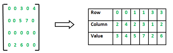
1. A sparse matrix is a matrix in which a large number of elements are zero. In contrast to a dense matrix, where most elements are non-zero, sparse matrices are more efficiently represented to save memory and computational resources. The representation of a sparse matrix as a 2D array involves storing only the non-zero elements along with their row and column indices.

Why Use Sparse Matrices?

1. Memory Efficiency: Sparse matrices can significantly reduce memory requirements by not storing zero elements, making them suitable for large matrices with a sparse distribution of non-zero values.

2. Computational Efficiency: Operations involving sparse matrices can be more computationally efficient, as only the non-zero elements need to be processed.

3. Reduced Storage Overhead: In dense matrices, the storage overhead of zero elements can be substantial. Sparse matrices help reduce this overhead.

4. Efficient for Certain Applications: Sparse matrices are commonly used in applications where the majority of elements are zero, such as graphs, network representations, finite element analysis, and certain mathematical models.

example:

0  0  3  0  4

0  0 5  7  0

0  0  3  0  0

0  2  6  0  0

2D array is used to represent a sparse matrix in which there are three rows named as 

• Row: Index of row, where non-zero element is located
• Column: Index of column, where non-zero element is located
• Value: Value of the non zero element located at index – (row,column)